Introduction
Structural Equation Modeling (SEM) is a comprehensive statistical technique used to analyze complex relationships among observed and latent variables. Combining elements of factor analysis and regression, SEM provides a powerful framework for testing hypotheses in social sciences, psychology, education, and business research.
This guide offers detailed, step-by-step instructions for conducting SEM in SPSS, with a focus on AMOS. By following this guide, you will gain a clear understanding of:
- What SEM is and its components.
- Key concepts such as latent variables, path analysis, and model fit.
- How to set up, run, and interpret SEM in AMOS.
- Best practices for ensuring your model meets statistical standards.
What is SEM?
Structural Equation Modeling (SEM) combines regression analysis and confirmatory factor analysis to simultaneously model relationships among variables. It is ideal for testing theoretical frameworks that involve direct, indirect, and mediating effects.
- Measurement Model: Specifies how latent variables are measured by observed indicators.
- Structural Model: Represents the relationships between latent variables and observed variables.
- Latent Variables: Abstract constructs measured indirectly via observed variables.
- Observed Variables: Directly measurable variables included in the analysis.
Why Use SEM?
Structural Equation Modeling (SEM) is a powerful tool because it enables researchers to test multiple relationships among variables simultaneously. Unlike traditional statistical techniques, SEM does not require separate tests for each relationship. Instead, it allows you to construct a single comprehensive model that incorporates all variables and their interactions. This capability is particularly beneficial for studies with complex theoretical frameworks, as it helps researchers analyze direct, indirect, and mediating effects within the same model, providing a holistic understanding of the data. For instance, SEM can simultaneously evaluate how a predictor variable influences several outcomes and how these outcomes, in turn, mediate or interact with other variables in the model.
Key Concepts in SEM
In SEM, understanding variable types is crucial for building accurate models. Variables are categorized based on their roles and measurement levels, which shape how they interact within the model.
- Observed Variables: These are directly measurable variables, often collected through surveys or assessments. For example, responses to a satisfaction survey represent observed variables that can provide insights into a latent construct like “satisfaction.”
- Latent Variables: Unlike observed variables, latent variables are abstract constructs inferred from multiple observed indicators. Examples include constructs like “intelligence,” which may be measured using various test scores.
- Exogenous Variables: Exogenous variables act as predictors within the model. They are independent and not influenced by any other variables in the SEM framework. For instance, factors like “education level” or “income” may serve as exogenous variables.
- Endogenous Variables: These are dependent variables influenced by either exogenous variables or other endogenous variables. An example would be “employee performance,” which may depend on both “job satisfaction” (endogenous) and “work environment” (exogenous).
Path Analysis
Path analysis is a foundational technique in SEM used to examine direct and indirect relationships among variables. Unlike basic regression analysis, path analysis involves multiple equations that explore how different variables interact. This method allows researchers to model relationships between observed variables, providing insights into causality and the pathways through which effects occur.
In SEM, path analysis extends to include latent variables, which represent abstract constructs measured indirectly. By integrating latent variables, path analysis becomes more comprehensive, allowing for a richer understanding of complex relationships.
Model Fit Indices
Model fit indices are critical for evaluating whether your SEM adequately represents the data. These indices compare the observed data with the hypothesized model to determine how well the model fits.
- Chi-square (χ²): This statistic tests the difference between the observed covariance matrix and the predicted matrix. A smaller chi-square value indicates a better fit, although it is highly sensitive to sample size.
- Comparative Fit Index (CFI): The CFI compares the fit of your model to a baseline model. Values greater than 0.95 are indicative of excellent fit.
- Root Mean Square Error of Approximation (RMSEA): RMSEA evaluates how well the model approximates the data. Values below 0.06 suggest a good fit.
- Tucker-Lewis Index (TLI): The TLI adjusts for model complexity. Values above 0.90 indicate an acceptable fit, with values above 0.95 being excellent.
- Standardized Root Mean Square Residual (SRMR): The SRMR represents the standardized difference between observed and predicted correlations. Values below 0.08 indicate a good fit.
- Goodness of Fit Index (GFI): The GFI measures the proportion of variance explained by the model. Values above 0.90 suggest a good fit.
- Adjusted Goodness of Fit Index (AGFI): The AGFI adjusts the GFI for the degrees of freedom in the model. Values above 0.90 are considered acceptable.
Interpreting Model Fit Indices
To ensure clarity, here is an updated reference table summarizing the acceptable ranges for key fit indices:
| Fit Index | Acceptable Range | Reference |
|---|---|---|
| Chi-square (χ²) | Non-significant | Hu & Bentler (1999) |
| CFI | > 0.95 | Bentler (1990) |
| RMSEA | < 0.06 | Browne & Cudeck (1993) |
| TLI | > 0.90 | Tucker & Lewis (1973) |
| SRMR | < 0.08 | Hu & Bentler (1999) |
| GFI | > 0.90 | Jöreskog & Sörbom (1984) |
| AGFI | > 0.90 | Tanaka & Huba (1985) |
Steps to Perform SEM in SPSS and AMOS
Performing SEM involves several steps, from preparing data to interpreting the results. This section details each step to ensure accuracy and clarity in your analysis.
Step 1: Prepare Your Data
Before running SEM, ensure your data is complete and meets the assumptions of multivariate analysis. This includes testing for normality, linearity, and the absence of multicollinearity. Organize your variables clearly and save the dataset in .sav format compatible with AMOS.
Step 2: Specify the Measurement Model
The measurement model defines how latent variables are measured by observed variables. Use confirmatory factor analysis (CFA) to validate the relationships between latent constructs and their indicators. Ensure factor loadings exceed 0.5 and are statistically significant to confirm the adequacy of the measurement model.
Step 3: Specify the Structural Model
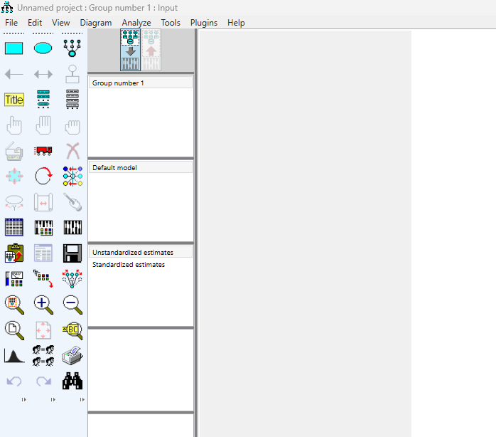
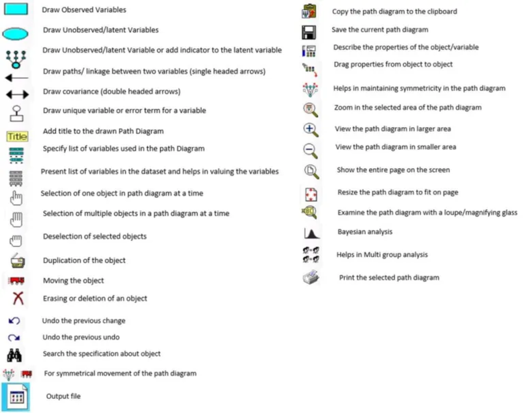
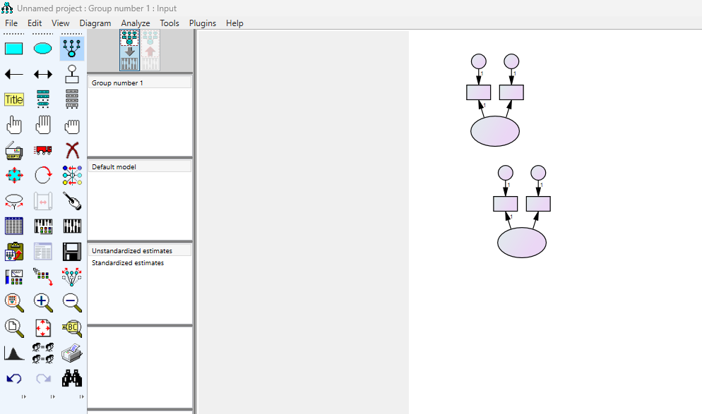
The structural model represents hypothesized relationships between latent variables. Use AMOS Graphics to create a path diagram. Add latent and observed variables, define paths, and include covariance relationships where appropriate. Specify constraints or fixed values where required.
Step 4: Estimate the Model
Choose Maximum Likelihood Estimation (MLE) as the default estimation technique. Run the model by clicking “Calculate Estimates” in AMOS. Evaluate the output for model fit indices, path coefficients, and residuals.
Step 5: Interpret the Results
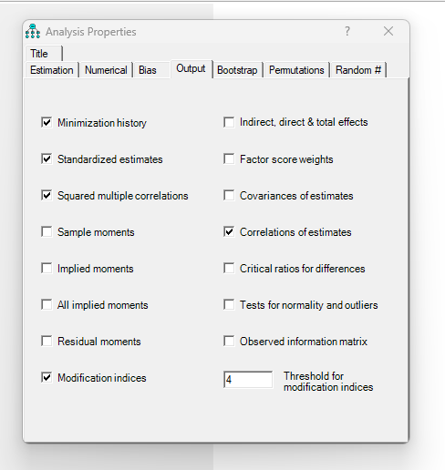
Examine the direct, indirect, and total effects reported in the output. Ensure the model meets acceptable thresholds for fit indices such as CFI, RMSEA, TLI, and SRMR. Use modification indices judiciously to refine the model while maintaining theoretical integrity.


